Guidesheet 4

Understanding Factorial Designs

Contents

Background

What are factorial designs?

What is a two-level factorial design?

Detecting curvature

What is a three-level factorial design?

What is a fractional factorial design?

Reference

Appendix

Background

We suggest you read our guidesheet titled 'Design of Experiments; Improving Your Products and Processes' (either the basic or advanced version) before reading "Understanding Factorial Designs' in order to understand the latter better. The latter is intended to give readers a basic understanding of what factorial designs are all about, including the types of factorial designs that are useful to manufacturing industries.

What are factorial Designs?

Most industrial and research experiments involve the investigation of many variables such as temperature, processing time, material type, humidity, etc. (henceforth referred to as 'factors') in order determine their effects on product quality and efficiency of manufacturing processes. For such experiments, the DOE technique known as factorial designs (also known as factorial experiments) are commonly used to design the experiments as well as to draw conclusions from the experimental results. Such designs enable us detect the effect of factors that interact, unlike the one-variable-at-a-time method.

In factorial designs,

• the number of levels for each of the factors is selected by the experimenter before the experiment is carried out.

• the number of possible combinations for the experiment is obtained by multiplying the levels of all of the factors together.

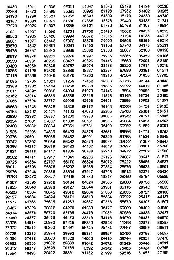
• whenever possible, the combination are then carried out in a random order. A random number table such as the one in the Appendix can be used for randomizing the order of the combinations.

When all of the combinations are carried out, the design is known as full factorial design (or simply factorial design). When only some of the combinations are carried out, the design is known as a fractional factorial design. The section titled 'What is a fractional factorial design?' touches on the latter.

What is two-level factorial design?

A two-level factorial design is a special type of factorial design. For such a design,

• the number of levels selected for each of the factors in the experiment is two.

• the number of possible combinations for the experiment is 2^k, where k is the number of factors.

• the combinations are carried out in a random order.

Since each of the factors is at two-levels, the number of combinations can be kept to a reasonable number as k increases. This can be seen in Table 1.

Table 1

A two-level factorial design is therefore useful when there are many factors to investigate in the experiment such as during process characterization, in which the objective is to determine the critical process factors. An actual example is given in the Appendix. However, if the process is already close to optimum conditions, the use of a factorial design that enables the critical factors to be studied over many levels may be more appropriate such as the use of a three-level factorial design. The latter is covered in the section titled 'Three-level factorial designs'.

Example

The simplest example of a two-level factorial design is when there are only two factors is the experiment.

• Let us label the factors as A and B; and the factor levels as A1, A2, B1, and B2.

• The number of possible combinations is 22 = 4. Table 2 lists the four combinations which are labeled as 'factor combinations'. The four facto combinations in Table 2 are said to be in 'standard order', that is the levels of A are alternated with each other in column 2 while the levels of B are alternated in pairs in column 3.

Table 2

• For each factor combination, an important measure of product quality or process efficiency or both such as yield, tensile strength, percent shrinkage, assembly time, cycle time, cost, etc. is obtained (henceforth referred to as 'response'). More than one product quality or process efficiency measures can be obtained.

• The experiment is repeated more than once in order to increase our confidence in the results of the experiment i.e. each of the factor combinations is performed more than once. Suppose the experiment is repeated twice. Since each of the factor combinations is performed twice, we will then have a total of eight runs for the experiment as shown in Table 3; the number of runs for each of the factor combinations being two.

Table 3

• To avoid any unknown systematic factors from affecting the results of the experiment, the order of performing the runs should be randomized. This is illustrated in the Appendix.

• The results of the runs are recorded as R1, R2, ...., R7 and R8 as can be seen in Table 3. The average of the results for the two runs at each of four factor combinations is then calculated and analyzed using either graphical or more formal statistical methods. The variability of the results for the runs at the four factor combinations can also be analyzed if one wishes to do so. The absolute value of the difference between : R1 and R2; R3 and R4; R5 and R6; and R7 and R8 can be used as a measure of the variability of the results (i.e. range value).

A practical example

Let us suppose that for Table 2,

• A and B represent pressure (in mm per second) and temperature (in degrees Celsius) respectively

• A1 = 140, A2 = 160, B1 = 30, B2 = 35

• response represents yield (in percent)

Suppose the yields are as shown in Table 4.

Table 4

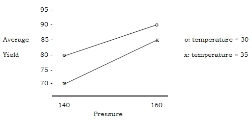
We will plot the average yields n Table 4 as shown in Figure 1.

Figure 1: Slight interaction between temperature and pressure

• increasing pressure corresponds to an increase in average yield for both temperature levels. Therefore, the higher pressure level should be used to increase the average yield regardless of the temperature level. However, the increase in average yield is greater for the case of the higher temperature level (15%) as compared to the case of the lower temperature level (10%). This suggests that there is slight interaction between temperature and pressure, but it doesn't affect the earlier advice to use the higher pressure level.

• best condition is when pressure is at the higher level and temperature is at the lower level for which the average yield is 90 percent. If such a yield is deemed adequate, the combination of higher pressure and lower temperature levels of 160 mm per second and 30 degrees Celsius respectively should be carried out several times in order to verify its yield before using this particular combination on the manufacturing floor. It is likely that average yields of more than 90 percent can be achieved with pressure levels that are higher than 160 mm per second and temperature levels that are lower than 30 degrees Celsius. Further experimentation is need to verify this.

Another scenario

Suppose the yields had turned out as in Table 5.

Table 5

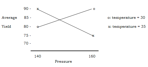
The plot of the average yields in Table 5 is shown in Figure 2.

Figure 2: Marked interaction between temperature and pressure

From the plot, it appears that

• pressure and temperature interact, as revealed by the crossing lines. At the lower temperature level, increasing pressure corresponds to an increase in average yield.  The higher pressure level should be used to maximize the yield at this temperature level.

• best condition is when pressure is at the tower level and temperature is at the higher level or when pressure is at the higher level and temperature is at the lower level, for which the average yield is 90 percent. We need to choose one of these two combinations, and to run it several times in order to verify its yield before using the combination on the manufacturing floor. The figure suggests that mid-pressure should also be investigated.

Detecting Curvature

When using two levels, it is assumed that the effect of the factors is approximately linear over the range they are tested at. That is, we assume there isn't any intermediate alue between the two levels that corresponds to the best condition. It this is a possibility, three levels should be investigated as illustrated below.

Example

Suppose three levels are to be used for pressure; 140, 150 and 160, since we suspect that the pressure value of 150 corresponds to the best condition. The number of levels for temperature is still two; 30 and 35. The number of possible combinations is now 3 x 2 = 6. Suppose the experiment is carried out twice, and that the order of the 6 x 2 = 12 runs are randomized. Suppose that the average of the yields from the two runs at each of the 6 factor combinations is as shown in Table 6.

Table 6

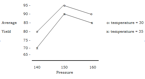
The plot of the average yields in Table 6 is as shown in Figure 3.

Figure 3: Curved relationship between pressure and yield

From the plot, it appears that

• for both temperature levels, here is a curved relationship between pressure and average yield, and that the best average yield corresponds to the intermediate pressure level.

• the lower temperature level seems to give better average yield than the higher temperature level. However, the difference in average yield between the two temperature levels at the intermediate and higher pressure levels are slightly smaller than that at the lower pressure level (i.e. 5% compared to 10%). This suggests that there is slight interaction between temperature and pressure but it doesn't affect our earlier advice to use the intermediate pressure level.

• the best condition is when pressure is at the intermediate level and temperature is at the lower level for which the average yield is 95 percent. Before using this combination of pressure and temperature on the manufacturing floor, it should be carried out several times in order to verify its yield.

What is a three-level factorial design?

For a three-level factorial design,

• the number of levels selected for each of the factors in the experiment is three.

• the number of possible combinations for the experiment is 3k, where k is the number of factors.

• the combinations are carried out in a random order.

Example

Suppose both pressure and temperature are to be tested at three levels; the levels being 140, 150, and 160 for pressure and 30, 35, and 40 for temperature. The number of possible combinations is now 3² = 9. Suppose the experiment is carried out twice, and that the order of the 9 x 2 = 18 runs are randomized. Suppose the average of the yields from the two runs at each of the nine factor combinations is as shown Table 7. As mentioned before, the advantage of using three levels is our ability to detect a curved relationship.

Table 7

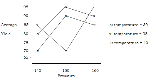
The average yields in Table  are plotted as shown in Figure 4.

Figure 4: Temperature-pressure plot

From the above plot,

• the curves cross indicating  a crucial interaction between temperature and pressure. This is why best average yield corresponds to the intermediate pressure level for both the low and high temperature levels but not for the low temperature level. For the latter, the intermediate pressure level produces the worst average yield.

• the best condition is when pressure is at the intermediate level and temperature is at the intermediate level. We need to choose which of these two to use, e.g. the cheaper combination, and to run it several times in order to verify its yield.

What is a fractional factorial design?

When the number of factors in the experiment (k) is large,

• the number of possible combinations increases rapidly. This is true even when the number of levels for each of the factors is two, as shown in Table 8.

Table 8

Fortunately, designs known as two-level fractional factorial designs can be used to obtain the information that we need without having to carry out all of the combinations. For instance, for an experiment involving 5 factors, each at two levels, only 16 out of the 32 possible combinations is needed in order to determine which are the critical factors as well as which pairs of factors interact. Montgomery (2000) including other DOE textbooks contains details of such designs including the method for selecting the combinations.

An actual example of a two-level fractional factorial design is given in the Appendix.
 

Table of Random Numbers
 

References

Montgomery, D.C. (1997) Design and Analysis of Experiments, Fourth edition, John Wiley & Sons Inc., Singapore.

Oh, S. H. (1995) Quality Control and Machine Vision System, Final Year Project Report, School of Industrial Technology, Universiti Sains Malaysia.

<< Appendix >>